The Problem & Dataset
What are we trying to do, and what data do we have to do it with?
What is SVHN and why does it matter?
SVHN stands for Street View House Numbers — a dataset of over 600,000 digit images cropped from street-level photos, originally assembled by Google to help automatically transcribe building numbers from Street View imagery.
If you know a building's address number and the street it's on, you can pinpoint its exact location. Automating that transcription at scale — reading the digits off millions of photos — is a real computer vision problem with real-world impact on mapping quality.
In this project we use a subset of the data: 120,000 images across train, validation, and test splits, each a 32×32 pixel greyscale crop centered on a single digit.
What does the data look like?
The data arrives as an HDF5 file — a structured binary format that stores large numerical arrays efficiently. Think of it as a very efficient spreadsheet for numbers. Each image is a 32×32 grid of pixel brightness values (0 = black, 255 = white). Each label is simply a number from 0 to 9 saying which digit is in the center of that crop.
One important design choice: the dataset came with a dedicated validation set of 60,000 images — larger than the training set. Rather than carving validation out of training data (which would waste 8,400 training samples), we used this pre-built split directly.
A surprise hiding in the images
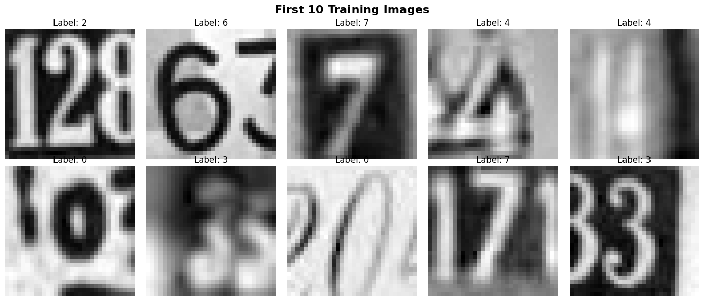
Each 32×32 crop was built by centering a window on the target digit in the original street photo. But the neighboring digits on either side naturally fall into frame too. An image labeled "2" might visually show "128" or "25" or "72".
The label only refers to the center digit — but the model has to figure that out on its own, from pixel patterns alone. This raised an interesting question explored later in Section 8: could we help the model focus on the center by mathematically dimming the edges before training?
Exploratory Data Analysis (EDA)
Before building any model, we examine the data to understand its structure, balance, and visual characteristics.
Are all digits equally represented?
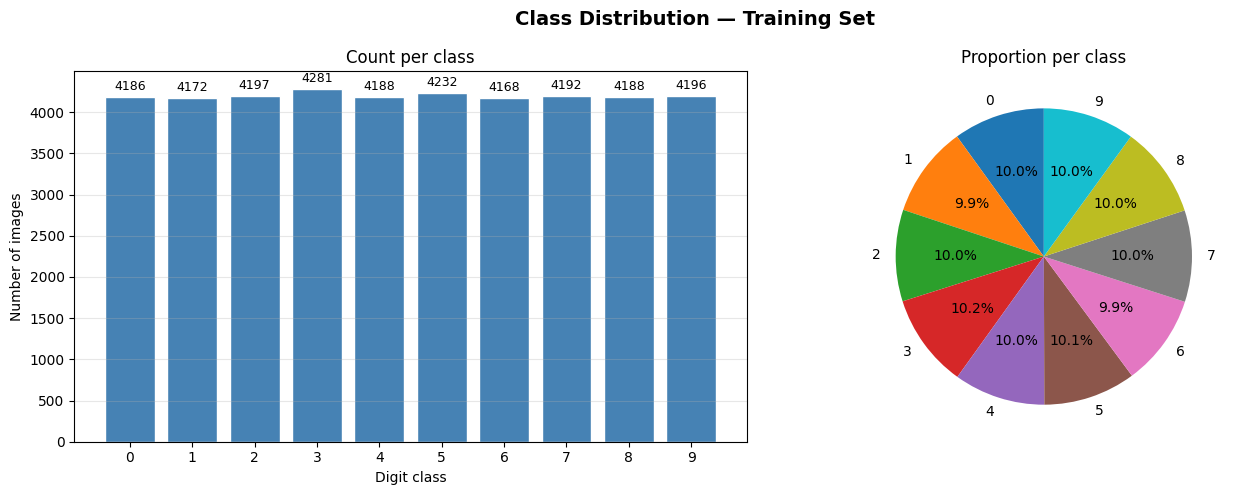
An imbalance ratio of 1.03 means the most common digit class has only 3% more images than the least common. That's essentially perfect balance. This matters because a heavily imbalanced dataset would bias a model toward predicting the majority class — making accuracy a misleading metric.
Here, accuracy is a trustworthy measure of real performance across all digits.
What does each digit actually look like?
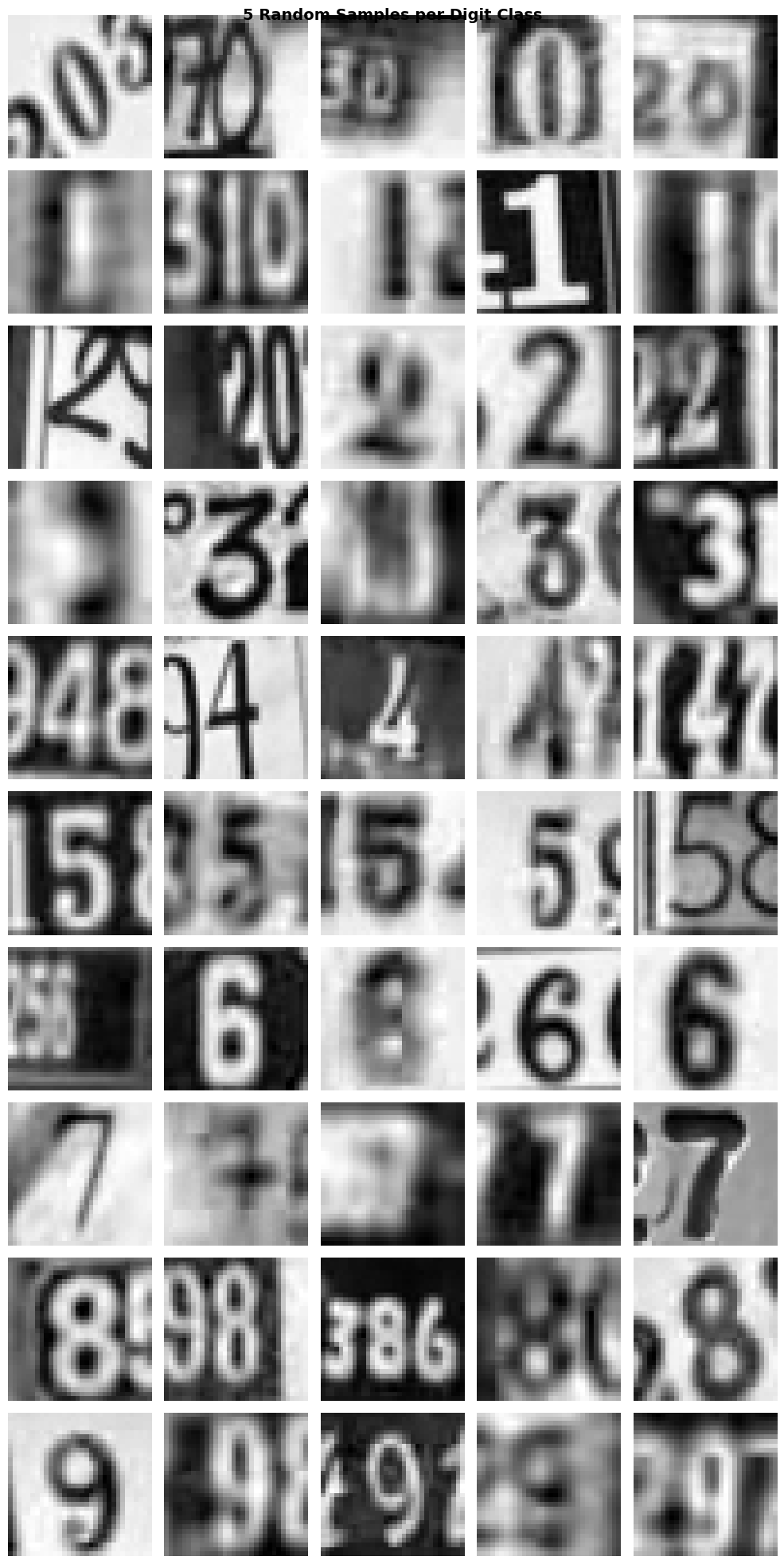
Each row shows five different examples of the same digit. The variation is striking: same digit, completely different fonts, sizes, angles, lighting, and backgrounds. A "7" might be bold or thin, tilted or upright, lit from the left or washed out by sunlight.
This is exactly why deep learning is needed here. A rule-based system ("a 7 has a horizontal bar at the top") would fail almost immediately. A neural network learns the statistical patterns that define a digit across all its real-world variations.
Pairs expected to cause the most confusion: 1 vs 7, 3 vs 8, 5 vs 6 — confirmed later in the confusion matrices.
Where does each digit's signal actually live in the image?
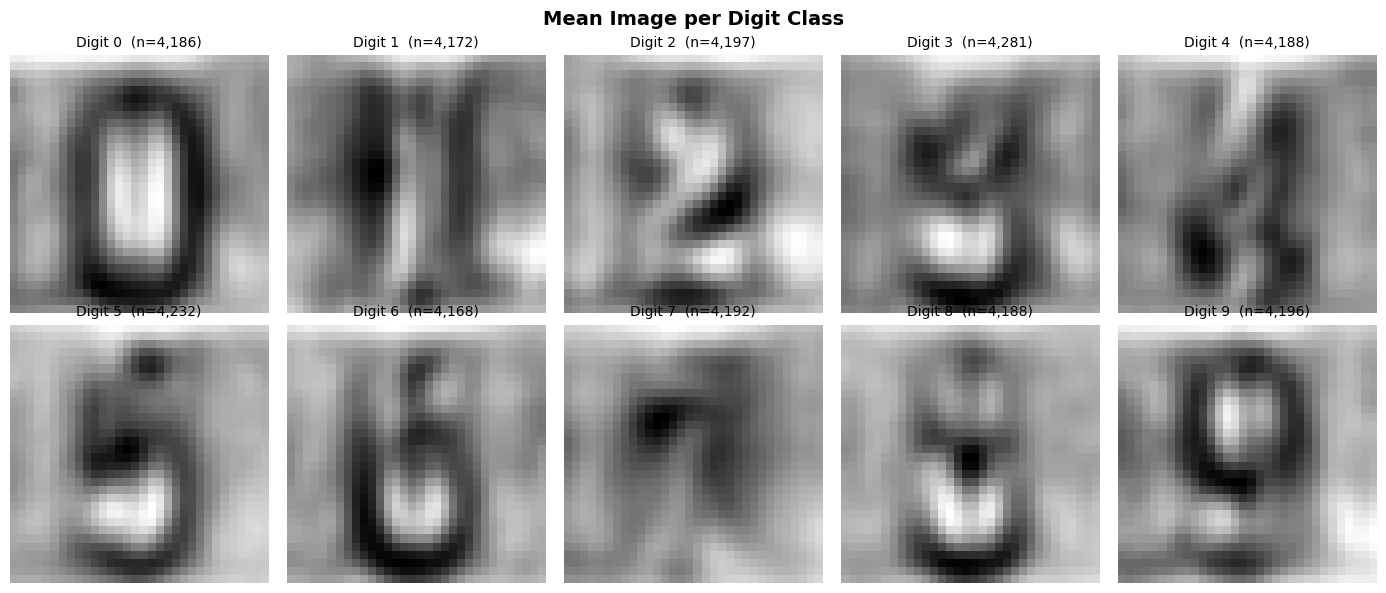
By averaging all images of each digit class, you get a "ghost image" that shows where strokes consistently appear. Bright areas = pixels that are usually bright for that digit. Dark areas = usually dark.
Two critical observations emerge:
1. Digit signal concentrates in the center. The mean images are brighter in the middle and fade toward the edges — confirming the neighboring-digit problem.
2. Background inversion is common. Some images have dark digits on a light background; others are the opposite. The mean image averages these out, producing a blurry center blob rather than a sharp digit shape. This inspired the spatial mask experiment in Section 8.
Data Preparation
Raw pixel data can't be fed directly to a neural network without some preparation steps.
Normalisation, reshaping, and one-hot encoding
Normalisation rescales pixel brightness from 0–255 down to 0.0–1.0. This keeps all inputs in the same range, which prevents the network's weights from being dominated by large pixel values and makes gradient descent more numerically stable.
Reshaping differs between ANN and CNN. An ANN receives a flat list of 1,024 numbers (32×32 unrolled). A CNN receives a 2D grid with an extra "channels" dimension — for greyscale images, that's always 1. Keeping the grid intact is what allows CNNs to detect spatial patterns like edges and curves.
One-hot encoding converts "label = 7" into a vector of ten zeros with a single 1 at position 7. The network then learns to output high probability at the correct position.
ANN Model 1 — The Baseline
We start simple: a fully-connected network that treats each image as a flat list of pixel values.
A small, shallow network — intentionally simple
An ANN (Artificial Neural Network) — also called a fully-connected or dense network — works by multiplying every input value by a learned weight, adding them up, and passing the result through an activation function. It does this in layers, each one building a more abstract representation.
The problem: when you flatten a 32×32 image into 1,024 numbers, you lose all spatial information. Pixel 100 no longer "knows" it's next to pixel 101. The network sees a long list, not a picture. This is the fundamental limitation we'll fix with CNNs later.
Training curves — learning progress over 20 epochs
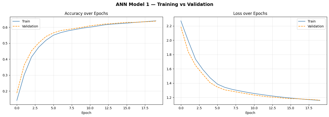
The training and validation curves track closely together — a good sign that the model isn't memorising the training data. However, 64% accuracy means the model gets roughly 1 in 3 predictions wrong. For 10 classes, random guessing would give 10% — so 64% is real learning, just not great learning.
The curves also plateau early, suggesting the model has hit its capacity ceiling. Adding more epochs won't help much — the architecture itself is the bottleneck.
ANN Model 2 — Deeper with Regularisation
More layers, more capacity, and two techniques to prevent memorisation: Dropout and BatchNorm.
A deeper network with regularisation layers
Dropout: during each training step, randomly "switches off" 40% of neurons. This forces the network to learn redundant representations — no single neuron can become essential. At test time, all neurons are active, but their outputs are scaled down. The result: better generalisation to new data.
BatchNorm (Batch Normalisation): after each layer, rescales activations to have zero mean and unit variance. This stabilises training, allows higher learning rates, and slightly regularises the network. The 64 non-trainable parameters store running statistics about the data distribution.
Training curves — 30 epochs
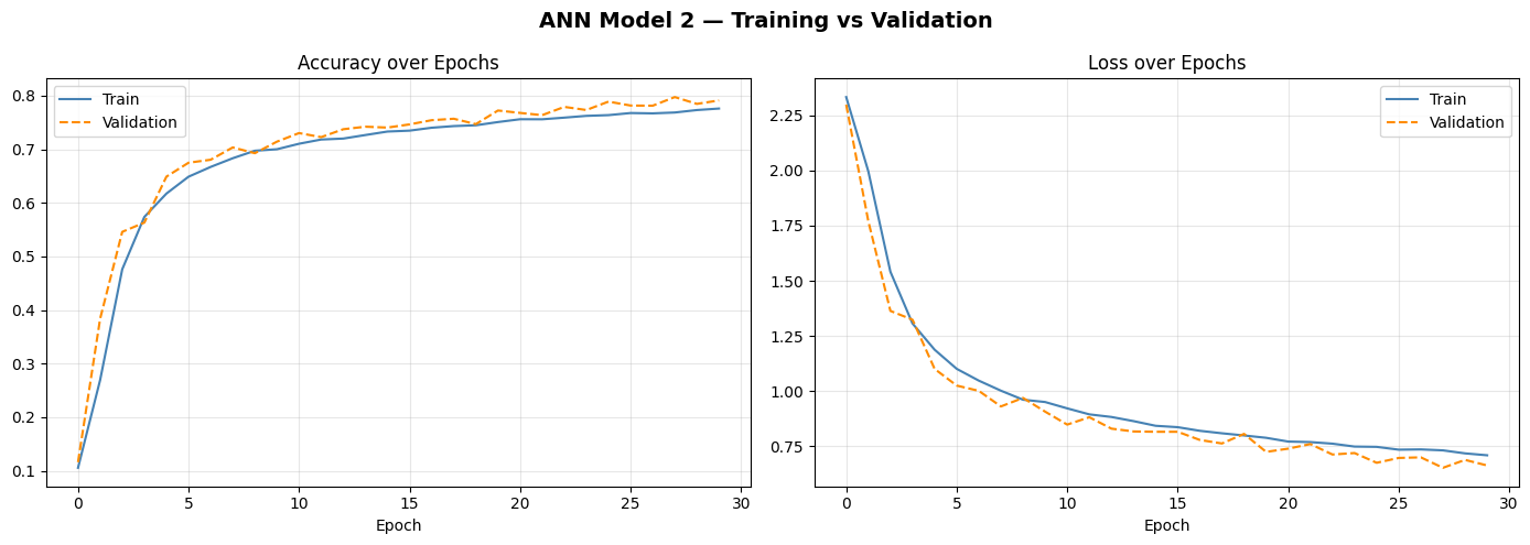
Interesting detail: validation accuracy slightly exceeds training accuracy (79.73% vs 77.59%). This can happen with Dropout — during training, neurons are randomly disabled, making training harder. At validation time, all neurons are active, giving the model full power. It's a sign Dropout is doing its job.
A significant improvement over Model 1 (+13.6 pts), but the ceiling is becoming visible. More depth helps — but without spatial awareness, even a very deep ANN has fundamental limitations.
Classification report & confusion matrix
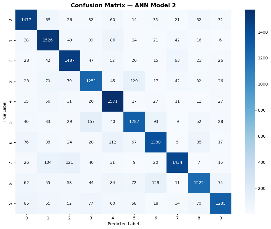
The confusion matrix is a grid where the bright squares on the diagonal = correct predictions. Off-diagonal bright spots = where the model confuses one digit for another. The most confused pairs: 3↔8, 5↔6, and 1↔7 — exactly as predicted from the sample images.
Precision: of all the times the model predicted "digit X", how often was it right? Recall: of all the actual "digit X" images, how many did the model catch? F1: the balance between the two. Digit 3 and 8 score lowest on both — the hardest pair to separate without spatial feature detection.
CNN Model 1 — Spatial Features Enter the Picture
Convolutional Neural Networks keep the 2D structure of the image intact and learn to detect visual features like edges, curves, and strokes.
Two convolutional blocks + a dense head
A convolutional layer slides a small filter (3×3 pixels) across the image and learns to detect a specific visual feature — an edge, a curve, a corner. Multiple filters run in parallel, each detecting something different. The network stacks these to build up from simple features (edges) to complex ones (digit shapes).
LeakyReLU: a variant of the standard activation function. Standard ReLU permanently kills neurons that produce negative values. LeakyReLU passes 10% of the negative signal through, keeping all neurons alive and trainable throughout.
MaxPooling: shrinks the image by half (2×2 → 1 pixel), keeping only the strongest signal in each region. This makes the network position-invariant — a "7" is still a "7" whether it's in the top-left or bottom-right of the crop.
Training curves reveal a classic overfitting problem
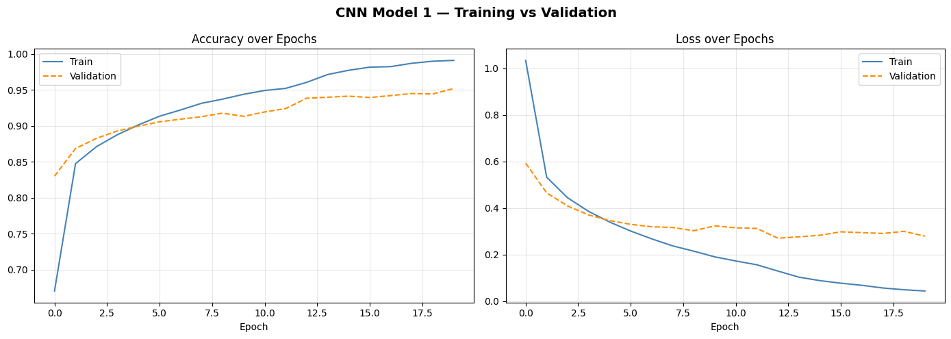
The model achieves 99% on training data but only 87% on unseen test data — an 11.78 percentage point gap. This is textbook overfitting: the model has memorised the training examples rather than learning generalizable rules.
The convolutional layers are fine — they share weights spatially, which naturally limits overfitting. The problem is the dense head: two fully-connected layers with no Dropout. Without regularisation, dense layers freely memorise. The fix: add Dropout to the dense head in Model 2.
CNN Model 2 — The Best Model
Deeper convolutions, BatchNorm throughout, Dropout in the dense head, and a model checkpoint to save the best weights. This is the final, production-quality model.
Four convolutional blocks with full regularisation
This model is deeper (4 conv blocks vs 2) but also smaller in total parameters (164K vs 267K) — because BatchNorm and Dropout do more work, the network doesn't need to be as wide. It's not about brute-force size; it's about learning efficiently.
Dropout(0.5) after Flatten: randomly drops 50% of the flattened feature map before the dense layers — this is the key fix from Model 1's overfitting. The dense head can no longer memorise.
A ModelCheckpoint callback saves the weights at the epoch where validation accuracy peaks — so even if the model starts to overfit in later epochs, we keep the best version.
Training curves — clean convergence, no overfitting

The training and validation curves run almost perfectly parallel — a hallmark of a well-regularised model. The gap between training and test accuracy has been cut from 11.78 to 4.04 points. That remaining gap is largely unavoidable: the test set contains genuinely harder images the model has never seen.
Validation accuracy (96.88%) slightly exceeding training accuracy (96.26%) is the Dropout effect again — the model is actually a bit held back during training but runs free at inference time.
Classification report & confusion matrix
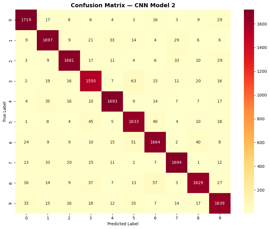
Compare these F1 scores to ANN Model 2: every single digit improved dramatically — from the 0.72–0.82 range to 0.90–0.95. The confusion matrix is almost entirely diagonal, meaning the model nearly always predicts the correct digit.
The hardest pairs (3 vs 8, 5 vs 6) still score slightly lower than the rest, but the gaps are now small. The spatial feature detection of CNNs — detecting the curved bottom of an 8 that a 3 doesn't have — directly addresses the root cause of those confusions.
Preprocessing Experiment: Data-Driven Spatial Mask
A bonus investigation: can we help the model by mathematically dimming the edge pixels (where neighboring digits appear) before training?
Building a mask from the data itself
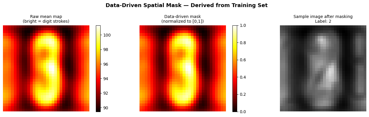
The mask is built entirely from the training data — no manual design, no geometric assumptions. By averaging all images, pixels that consistently carry digit information (the center) stay bright. Pixels dominated by neighboring digits or background (the edges) become dimmer.
The center pixel gets a weight of 0.86 while corner pixels get only 0.33 — the mask is 2.6× stronger in the center. When multiplied against input images, edge information is dampened before the network ever sees it.
Raw inputs: 92.22% — Masked inputs: 87.11%
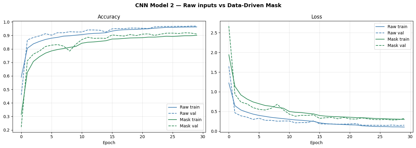
The mask made things worse. Three reasons why:
1. It clips real signal. The mean image shows where digits appear on average — but 69.4% of images were already background-inverted before averaging. Individual digits still vary in position. The mask dims pixels that sometimes carry genuine information.
2. CNN Model 2 already learned this. Getting 92.22% on raw inputs means the conv filters independently developed center-focus during training. The mask makes explicit what the CNN already learned — just less precisely.
3. Preprocessing is irreversible. Once a pixel is multiplied by the mask weight, that information is gone permanently. A CNN trained on raw inputs can choose to ignore edge pixels case-by-case. The masked CNN can't choose to recover them.
Takeaway: for this architecture and dataset, the CNN is a better spatial filter than anything that can be designed manually. Raw inputs win.
Full Model Comparison
All four models, side by side.
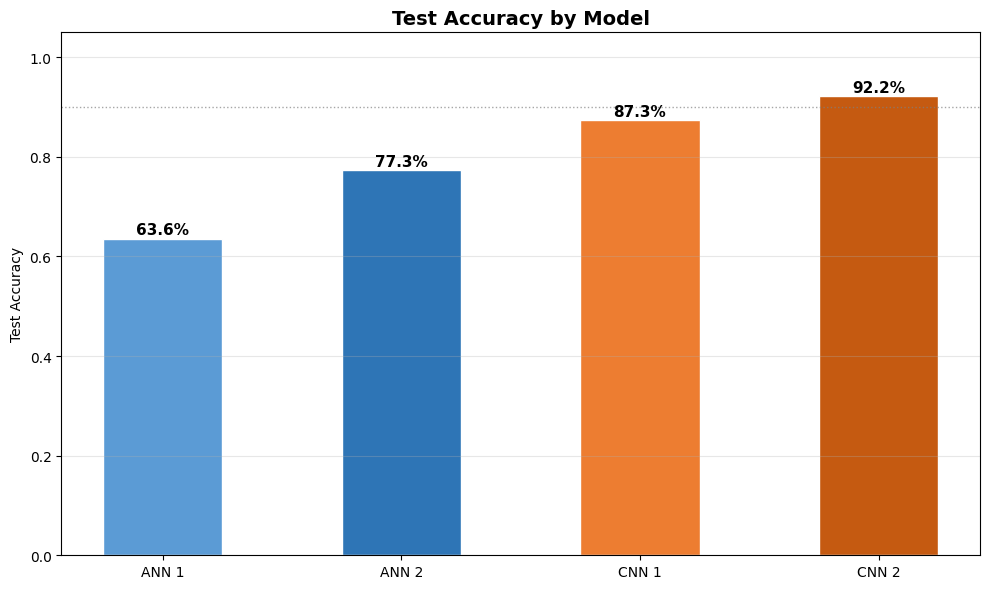
All models ranked by test accuracy
| Model | Architecture | Train Acc | Val Acc | Test Acc | Key Characteristic |
|---|---|---|---|---|---|
| ANN Model 1 | 64→32→10 | 64.02% | 63.86% | 63.57% | Shallow baseline — no spatial awareness |
| ANN Model 2 | 256→128→64→32 + Dropout + BN | 77.59% | 79.73% | 77.33% | Deeper — still no spatial structure |
| CNN Model 1 | 2 conv blocks | 99.08% | 95.17% | 87.30% | Spatial features work — overfits without Dropout |
| CNN Model 2 | 4 conv blocks + BN + Dropout | 96.26% | 96.88% | 92.22% | Best — depth + regularisation + clean gap |
Error Analysis — Understanding the Mistakes
Metrics tell us how many errors. Inspecting the actual wrong predictions tells us why — which is far more actionable.
Misclassified images — what went wrong?
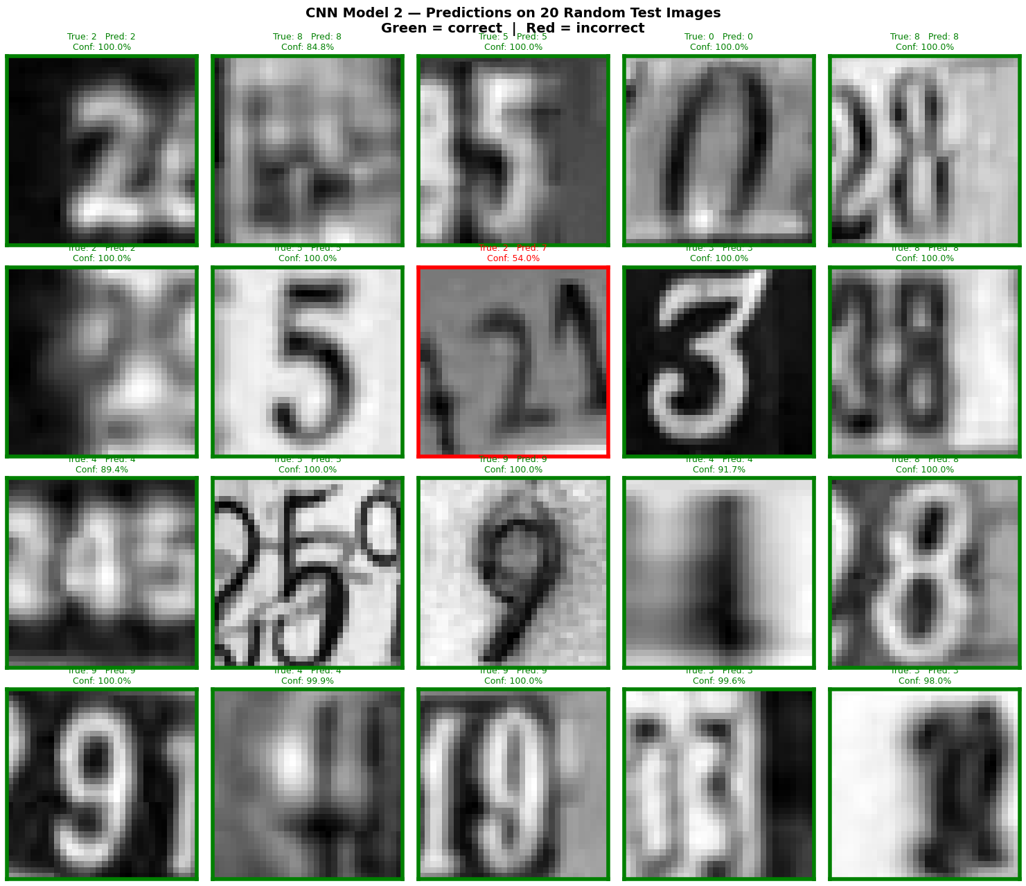
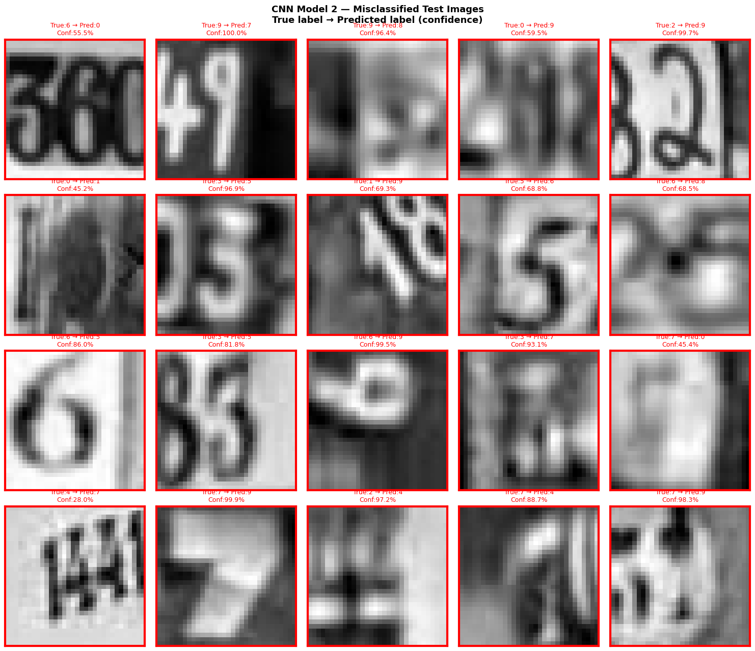
Of the 1,401 errors, most fall into two categories:
Genuinely ambiguous images — digits that look visually similar in real photos (1 vs 7, 3 vs 8, 5 vs 6). Even a human might struggle with some of these. The model's confusion is appropriate.
High-confidence wrong predictions — these are the most concerning. A model that predicts "1" with 92% confidence but the true label is "4" is being overconfident. These cases are worth investigating because they represent a failure of calibration, not just capacity.
The error analysis is not just a performance metric — it's a debugging tool that tells us what kinds of images to add or augment in future training runs to close specific gaps.
Final Conclusions
Eight things this project proves, empirically
1. CNNs massively outperform ANNs (+14.89 pts on test accuracy). ANNs flatten the image and throw away all spatial structure before processing. CNNs keep it, using filters that detect edges, strokes, and curves. That difference alone accounts for most of the accuracy gap.
2. Deeper models with regularisation consistently win. In both families, the deeper regularised model beat the shallower one. Depth gives capacity; Dropout and BatchNorm make sure that capacity generalises rather than memorises.
3. CNN Model 1 showed exactly why Dropout in the dense head matters. Without it: 99.08% train, 87.30% test — an 11.78 point gap. Textbook overfitting. Adding Dropout(0.5) in Model 2's dense head cut that gap to 4.04 points.
4. LeakyReLU matters in conv layers. Standard ReLU permanently kills filters that produce negative pre-activations. LeakyReLU(0.1) keeps a 10% gradient so no filter ever gets stuck during training.
5. Use the provided validation set — don't cut into training data. The H5 file came with 60,000 dedicated validation images. Using validation_split=0.2 instead would have wasted 8,400 training samples for no reason.
6. A clever preprocessing mask is still worse than a well-trained CNN. The spatial mask scored 87.11% vs 92.22% for raw inputs — a −5.11% drop. CNN Model 2 already learns center-focus implicitly. Preprocessing is irreversible; neural networks learn.
7. Fewer parameters + better architecture > more parameters + poor design. CNN Model 2 (164K params) outperforms CNN Model 1 (267K params) by 4.92 points. Regularisation is more valuable than raw capacity.
8. The remaining errors make sense. 1,401 out of 18,000 wrong (7.8% error rate). Error analysis shows most wrong predictions are on genuinely hard images — the model fails on the cases where a human would also hesitate.